Practical Methods and Workarounds for Calculating Geometric Mean

by Dr. Joe Costa

Definition of Geometric Mean

Means are mathematical formulations used to characterize the central tendency of a set of numbers. Most people are familiar with the “arithmetic mean”, which is also commonly called an average. Geometric mean has the specific definitions below, and has utility in science, finance, and statistics.

Mathematical definition: The nth root of the product of n numbers.

Practical definition: The average of the logarithmic values of a data set, converted back to a base 10 number.

Geometric Means for Water Quality Standards

Many wastewater dischargers, as well as regulators who monitor swimming beaches and shellfish areas, must test for and report fecal coliform bacteria concentrations. Often, the data must be summarized as a “geometric mean” (a type of average) of all the test results obtained during a reporting period. Typically, public health regulations identify a precise geometric mean concentration at which shellfish beds or swimming beaches must be closed.

A geometric mean, unlike an arithmetic mean, tends to dampen the effect of very high or low values, which might bias the mean if a straight average (arithmetic mean) were calculated. This is helpful when analyzing bacteria concentrations, because levels may vary anywhere from 10 to 10,000 fold over a given period. As explained below, geometric mean is really a log-transformation of data to enable meaningful statistical evaluations.

Other Uses of Geometric Means

Besides being used by scientists and biologists, geometric means are also used in many other fields, most notably financial reporting. This is because when evaluating investment returns as annual percent change data over several years (or fluctuating interest rates), it is the geometric mean, not the arithmetic mean, that tells you what the average financial rate of return would have had to have been over the entire investment period to achieve the end result. This term is also so called the Compound Annual Growth Rate or CAGR. Population biologists also use the same calculation to determine average growth rates of populations, and this growth rate is referred to as the Intrinsic Rate of Growth when the calculation is applied to estimates of population increases where there are no density-dependent forces regulating the population.

Financial Return Calculation

For financial investment return calculations, the geometric mean is calculated on the decimal multiplier equivalent values, not percent values (i.e., a 6% increase becomes 1.06; a 3% decline is transformed to 0.97. Just follow the steps outlined in the section below titled Calculating Geometric Means with Negative Values).

The equation is also flipped around when calculating the financial rate of return if you know the starting value, end value, and the time period. This equation is used in these cases when the average rate of return is needed (or population growth rate):

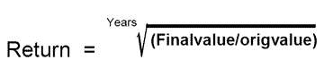
Note: If you subtract 1 from the equation above, this is your compound interest rate. To use this equation, if years=5, this is the “fifth root”, which is the same as raising to the power of 1/5 or 0.2).

Problem submitted by a student:
“A recent article suggested that if you earn $25,000 a year today and the inflation rate continues at 3 percent per year, you’ll need to make $33,598 in 10 years to have the same buying power. … Confirm that this statement is accurate by finding the geometric mean rate of increase”

Solution using a formula in Excel:   =Power(33598/25000,.1)=1.03

When to Use or Not Use Geometric Mean

Geometric mean is often used to evaluate data covering several orders of magnitude, and sometimes for evaluating ratios, percentage changes, or other data sets bounded by zero. If your data covers a narrow range (I have seen it stated that the largest value must be at least 3x the smallest value for geometric mean to be applicable), or if the data is normally distributed around high values (i.e. skew to the left), geometric means (log transformations) may not be appropriate. Instead of using logarithmic transformations, biologists and scientists in other fields may use other types of data transformations. For example, the Arcsine Transformation (take the arcsine of the square root of the number) is commonly use on proportions data, where the values are bounded by 0 and 1 (especially when the values are close to boundary conditions). A fuller explanation of data transformations used by biologists can be found on Dr. John McDonald’s website. Do not use geometric mean on data that is already log transformed such as pH or decibels (dB).

Geometric Mean Calculation

How do you calculate a geometric mean? The easiest way to think of the geometric mean is that it is the average of the logarithmic values, converted back to a base 10 number.

However, the actual formula and definition of the geometric mean is that it is the nth root of the product of n numbers, or:
Geometric Mean = n-th root of (X₁)(X₂)…(X_n)

Where X₁, X₂, etc. represent the individual data points, and n is the total number of data points used in the calculation.

If this is the definition of geometric mean, why is my first statement true, that geometric mean is really the average of the log values?

Consider this example. Suppose you wanted to calculate the geometric mean of the numbers 2 and 32.
This simple example can be done in your head. First, take the product; 2 times 32 is 64. Because there are only two numbers, the nth root is the square root, and the square root of 64 is 8. Therefore the geometric mean of 2 and 32 is 8.

Now, let’s solve the problems using logs. In this case, we will convert to base-2 logs so that we can solve the problem in our head (in fact, any base could be used). Converting our numbers, we have:

2=2¹
32=2⁵
2¹ x 2⁵ = 2⁶ (=64)
the square root of 2⁶ is 2³ (=8)

Of course, the short cut to solve the problem is to take the average of the two exponents (1 and 5) which is 3, and 2³ is 8.

Mental Math Problem: Can you calculate the geometric mean of these 5 numbers, in your head?

2³, 2⁵, 2⁸, 2³, 2¹ (These values of course equal 8, 32, 256, 8, and 2)
(Hint: The 5 exponents add up to 20.) Click for the answer.

From the discussion above, you can see that the calculation of the Geometric Mean can be performed by either of two procedures on a calculator, depending upon which functions are available. Computer-based spreadsheet programs like Excel have built geometric mean functions, and in general you should use these (see below) to save time if a computer with the appropriate software is available.

Calculation Procedure 1: Multiply all of the data points, and take the nth root of this product.

Example:
Suppose you have this beach monitoring data from different dates:
(data are Enterococci bacteria per 100 milliliters of sample)

   6 ent./100 ml
50 ent./100 ml
9 ent./100 ml
1200 ent./100 ml

Geometric Mean = 4th root of (6)(50)(9)(1200)

   = 4th root of 3,240,000

Geometric Mean = 42.4 ent./100 ml

On a good scientific calculator, you would multiply the numbers together, press equal, then the root key, then the number 4 to get the forth root (or enter 0.25 with the exponent key on the last part).

Calculation Procedure 2: Take the average of the logs, then convert to a base 10 number

Of course, many calculators do not have a root key that allow the calculation of any root, so you must use the logarithm function, which is typically more widely available on calculators. To use this calculation procedure, you must have a calculator which will give logarithms (log or ln) and anti-logarithms (exp or e).

The first step in calculating the Geometric Mean using this method is to determine the logarithm of each data point using your calculator. Next, add all of the data point logarithms together and divide this sum by the number of data points (n). In other words, take the average of the logs. Next, convert this log average back to a base 10 number using the antilogarithm function key on the calculator.

Example (using previous data):

   log 6= 0.77815
log 50= 1.69897
log 9= 0.95424
log 1200= 3.07918

Sum= 6.51054

The logarithm of the Geometric Mean is 6.51054/4 = 1.62764 (the average of the logs)

From your calculator, determine the number whose logarithm is 1.62764 (use the antilogarithm key), and you will find that the Geometric Mean = 42.4 ent./100 ml

This process works whether or not you use natural logs (“ln” key) or base 10 logs (“log” key). That is, on your calculator you could do ln(x₁), ln(x₂), etc. then use the ‘ex’ key on the average of the logs, or you would do log(x₁), log(x₂), etc. then use the ’10^x‘ key on the average of the logs. (key names may vary among calculators).

Incidentally, for this example data set, the arithmetic mean (average) of the four data points is:

Arithmetic Mean = (6 + 50 + 9 + 1200)/4 = 1265/4
Arithmetic Mean = 316.3 colonies/100 ml

The geometric mean is always less than the arithmetic mean (except of course if all the data points have an identical value).

On most scientific calculators your key sequences to calculate the geometric mean would be:

enter a data point,
press either the Log or ln function key,
record the result or store it in memory,
calculate the mean or average of these log values,
calculate the antilog value of this mean (’10^x‘ key if you used ‘Log’ key, ‘e^x‘ key if you used ‘ln’ key)

Calculating Geometric Means in Spreadsheets

Rather than using a calculator, it is far easier to use spreadsheet functions. For example, in Microsoft Excel™ the simple function “GeoMean” is provided to calculate the geometric mean of a series of data. For example, if you had 11 values in the range A1…A10, you would simply write this formula in any empty cell: ‘=geomean(A1:A10)’. In Corel Quattro™ spreadsheets, the function is ‘@geomean(A1..A10)’. In both programs, you can enter values directly inside the parentheses (x1,x2,x3) instead of referencing a range of cells.

The following formulas are equivalent in Excel:

=GEOMEAN(datarange)
=POWER(PRODUCT(datarange),(1/count(datarange)))
{=EXP(AVERAGE(LN(datarange)))}

The curly brackets in the last formula means this is an array formula, and it is created by simultaneously pressing CTL-SHIFT-ENTER after you type in the formula. You can, of course, use a defined range name in these formulas in Excel and other spreadsheet programs.

Calculating Geometric Means with Zero Values

The calculation of the Geometric Mean may appear impossible if one or more of the data points is zero (0). Often these zero values are really less than some the limit of detection, and are referred to as censored data. Below detection limit values are sometimes substituted with zero (not useful for geometric means), half the limit of detection, the limit of detection divided by the square root of two, the detection limit itself, or some other value (Kayhanian et al., 2002). Sometimes the value one (or another constant) is added to all values to eliminate zeros or negative values, or in the case of frequency data, by adding 0.5 to all values (McDonald, 2009). Some regulatory agencies require a particular substitution methodology. For example, the US Food and Drug Administration in its shellfish sanitation program regulations requires the substitution of a value that is one significant digit less than the detection limit [i.e. “less than 2” becomes “1.9”]. All these substitutions techniques preserve information that would otherwise be lost in a statistical evaluation. Because of how geometric mean is calculated, the precise substitution value often does not appreciably affect the result of the calculation, but there are exceptions. To see how to construct a spreadsheet formula to change censored values to one significant digit, see the Spreadsheet Tips section below.

Here is an example with a non-detect (and assuming the detection limit was 2 bacteria per 100 milliliters):

1100
0 (“less than 2”)
30
13000

Geometric Mean = 4th root of 1100 X 1 X 30 X 13000

= 4th root of 429,000,000

Geometric Mean = 143.9

Incidentally, substituting 1.9 for the less than value results in a geometric mean of 169.0, which is nearly statistically different (alpha=0.05) using a t-test using the substituted value 1.0 (half the detection limit). See additional comments in the bacteria data section below.

Debate on the use of substitutions of below reporting limits and other censored data

Many statisticians have criticized common procedures for providing substituted values for non-detects or below-reported-limits value data. Other alternatives, such as “delta log-normal models” have also received criticism and even legal challenges when applied to regulatory discharges permits. These problems and alternative analysis strategies are presented in Helsel (1990, 2005) and EPA (2002). These references also contain useful citations to other publications.

Statistical tests on bacterial data

All statistical tests used to evaluate variable bacterial data (i.e. a range of values over orders of magnitude) should be employed using the means, variances, or standard deviations of the log-transformed data. However, a special problem is created when reporting standard deviations of log data. That is because plus or minus (+/-) a log constant creates unequal error bars when converting back to base 10 (see note below on plotting geometric means).

For example, for the geometric mean of 10, 100, and 1000, your statistics (using base 10) is to take the mean and standard deviation of 1, 2, 3. Mean=2, STDEV=1, so it is 2+/-1. Converting back to base 10, your geometric mean is 100 +900/-90 (unequal upside and downside error bars).

To overcome other log transformation problems, values less than detection limits should be replaced with non-zero value to avoid log of zero errors. As noted above, certain regulatory programs, like the US FDA requires the substitution of a number one significant digit less than the detection limit [i.e. “less than 2” becomes “1.9”], or one significant digit larger for exceedances [i.e. “Greater than 1600” becomes “1700”] under their shellfish sanitation program regulations. Other agencies have required models to predict the variance of these below-reported-limits data.

Another special problem that exists with bacteria testing is that bacterial plates can be inundated with bacteria so that bacteria colony forming units are expressed as exceeding a certain number. These “greater than” values are similarly converted for geometric mean calculations (FDA requires conversion to the next significant digit (“>1200” becomes “1300”). Regulatory programs like these also have water quality standards that incorporate median values and 90th percentile values because of concerns about possible non-normal distributions of even the log-transformed data.

The calculated means and variances of log-transformed data can be plugged into a t-Test to evaluate whether there is a statistical between two stations. To answer the question whether there is a statistical difference among three or more stations, use an ANOVA test. When analyzing log-transformed data, you may be surprised to find that two sites with remarkably different arithmetic means may be not statistically different from one another. The substitution values for non-detects can sometimes affect the outcomes of statistical tests, especially in cases where a large percentage of the data are non-detect or zero. Helsel (1990, 2005) describes a variety of tests and approaches that are more robust and valid in evaluating this type of data.

Plotting log transformed data

It is relatively easy to plot log-transformed data in spreadsheet programs. When graphing standard deviations or standard errors around a mean, your error bars will be of equal size above and below the mean if you plot on log paper or apply a log scale in a spreadsheet program. However, the error bars will be unequal (different upside and downside standard deviations) if the y axis is not log transformed.

Calculating Geometric Means with Negative Values

Like zero, it is impossible to calculate Geometric Mean with negative numbers. However, there are several work-arounds for this problem, all of which require that the negative values be converted or transformed to a meaningful positive equivalent value. Most often, this problem arises when it is desired to calculate the geometric mean of a percent change in a population or a financial return, which includes negative numbers.

For example, to calculate the geometric mean of the values +12%, -8%, and +2%, instead calculate the geometric mean of their decimal multiplier equivalents of 1.12, 0.92, and 1.02, to compute a geometric mean of 1.0167. Subtracting 1 from this value gives the geometric mean of +1.67% as a net rate of population growth (or in financial circles is called the Compound Annual Growth Rate-CAGR).

Incidentally, if you do not have a negative percent value in a data set, you should still convert the percent values to the decimal equivalent multiplier. It is important to recognize that when dealing with percent values, the geometric mean of percent values does not equal the geometric mean of the decimal multiplier equivalents.

For example:

Geometric mean of [12%, 4%, 2%] does not equal the Geometric mean of [1.12,1.04,1.02].

4.6% does not equal 5.9%

Calculating Geometric Means with Both Large Negative and Positive Numbers Combined

I have received a number of queries, particularly from those analyzing gene block microarray data sets, about how to calculate geometric means on data sets that include both very large and very positive numbers. The analysis of data to evaluate the similarity of gene blocks is a complex topic and the statistics of this field is evolving, and you should perform an Internet search to find the latest thinking on this topic.

However, in principal, comparing data sets consisting of very large negative and positive numbers together is an easy matter, and all that is required is to temporarily suspend the negative signs of the data.

Consider, for example, two sets sample data sets as follows:
|    A= {-5,-3,-2, 3} and B={-1, 0, 2, 4}

The arithmetic mean of data set A is -1.75, and the arithmetic mean of data set B is +1.25. A simple Student’s t-test (assuming alpha=0.05 and equal sample variances) would suggest these samples are not statistically different from one another.

This approach would be no different than if you were to calculate geometric mean in these two data sets:
|    A’={-100000, -1000, -100, 1000} and B’={-10,1,100,10000}

If you were to take off the negative signs, take the log, then add the negative sign back on, you could then compare the means of the A’ and B’ data sets. In fact, you might have noticed that data sets A and B are really the log (base 10) transformed data sets A’ and B’ (after suspending then adding back the negative signs). You might therefore conclude that A’ and B’ are not statistically different samples using the same t-test.

Incidentally, in a spreadsheet, you can calculate the average of the logs of a set of large negative and positive numbers using this array formula (this example is base 10):
{=AVERAGE(SIGN(rangename)*LOG(ABS(rangename),10))} = -1.75 for A’.

The actual geometric mean of the values is calculated by the array formula:
{=SIGN(range)*GEOMEAN(ABS(range))} = -1778.28 for A’.

Don’t type in the curly brackets in the above formulas, type the formula, then press CTL-SHIFT-ENTER.

Of course, like any other statistical analysis, you have to make sure you have not violated the assumptions of the statistical test (in this case you must assume the log transformed data is normally distributed, and the sample variances were equal).

Geometric Mean of Grouped Data

A student recently posed this question: How do you calculate the geometric mean on grouped data? That is to say, when the data exists as a data range and frequency, what formula do you use?

As per the discussion above, there are two ways to approach this problem:

Method 1: (hardest for grouped data): Calculate the product of all the values in the data set (frequency of each mid-point value), then take the nth root of the product, with n being equal to the cumulative frequency.

Method 2: (easiest for grouped data): Calculated the average weighted mean of the logarithm of each mid-point value, then convert this mean value back to a base 10 number.

These two statements are best illustrated by the sample data set in the table below.

	Arithmetic Mean Calculation			Geometric Mean Calculation (Meth. 1)
range	frequency	midpoint	freq x mid	ln(midpt)	freq x ln(midpt)
10 to >=20	3	15	45	2.708	8.124
20 to >=30	9	25	225	3.219	28.970
30 to >=40	5	35	175	3.555	17.777
Total	17		445		54.871
		arithmetic mean=	26.176	arithmetic mean of weighted ln=	3.228

Using Method 1, you would take the 17th root of the product
15 x 15 x 15 x 25 x 25 x 25 x 25 x 25 x 25 x 25 x 25 x 25 x 35 x 35 x 35 x 35 x 35,

which is also equal to 25.221.

In a spreadsheet, you would type this formula:
=((15^3)*(25^9)*(35^5))^(1/17)

As you might imagine, if you have large mid-point values or large frequencies, your calculator or spreadsheet program could not compute the formula because the intermediate numbers are impossibly large, and the result would be an error. To calculate geometric mean in these cases, you must use Method 2. You might also consider the spreadsheet “array formula” method in the “Excel #Num! overflow error” callout box above. If your grouped data includes large negative numbers, you have no choice but think of a clever transformation to make the values positive and use Method 2.

For Method 2, as shown in the table above, you would calculate the weighted mean of the natural logarithms of the mid-point values, which in this case is 3.228. When the value is converted back to base 10, the geometric mean is 25.221.

Interestingly, this problem is quite similar to one faced by the Buzzards Bay NEP, in evaluating the extent of oiling from an oil spill. In this case, the data consisted of an average width and the length of the beach. For example, 1500 ft. of beach may have had between 0 and 5 foot-wide band of oil, 10,000 feet may have been documented to have a band of oil between 5 and 10 ft., etc. The length of beach oiled became the frequency for the interval.

Whether geometric mean is an appropriate metric for evaluating this type of data, or any other data set, always needs to carefully considered.

Working Backward

This following problem was posed by a student:

If Geomean(8,a)=12, what is a?

The question can be most easily be rephrased using the nth root definition of geometric mean. That is:

square root of (8 x a)=12

solve first by squaring both sides:
(8xa)=144
a=144/8 = 18

Using logs, the mathematical solution is:

First express the problem as the mean of logs:
(ln(8)+ln(a))/2 =ln(12)

Solving:
ln(8)+ln(a) =2 x ln(12) ===> ln(a)=(2 x ln(12))-ln(8) ===>a =exp((2 x ln(12))-ln(8)) ===> a=exp(2.8904) ===> a=18

Exceedances and Too Numerous to Count (TNTC)

In the case of reporting bacteria geometric means, problematic data include not only samples less than the limit of detection, but also those samples where colony forming units (CFUs) are too numerous to count. The upper limit in the number of bacteria colonies that can be counted on an incubation plate depends on a number of factors that relate to merging of colonies, swarming, and the size of the plate. How these plates are reported depends on method used and reporting protocols. For example, most agencies that issue discharge permits discourage or prohibit the use of TNTC. Instead they require the reporting of values as “> x.” For example, under ASTM (7), if with a 1:10 dilution, only 200 CFU could be meaningfully counted, the results would reported as >2,000 CFU/ml. In the case of discharge monitoring of under EPA’s NPDES program, where monthly geometric means are reported, the “>” sign is stripped and the value used in the geometric mean calculation (e.g. Florida DEP, 2012). In the FDA shellfish sanitation program protocols, “individual plates which are too numerous to count (TNTC) are considered to have >100 colonies per plate. A sample containing “TNTC” plates is collectively rendered as having a count of 10,000″ (FDA National Shellfish Sanitation Program Guide for the Control of Molluscan Shellfish 2007 ).

Spreadsheet Tips

If your data contains censored (> and <) data, you could consider using one of these formulas (where the data is in column c):

If you wanted to convert values by a certain multiple (half for < data and double for > data in this example), you could use this formula:

=IF(LEFT(C1,1)=”<“,VALUE(MID(C1,2,20))/2,IF(LEFT(C1,1)=”>”,VALUE(MID(C1,2,20))*2,C1))

If you wanted to use the US FDA censored data protocol (decreasing or increasing by one significant digit), this complicated formula should work:

=IF(LEFT(C1,1)=”<“,VALUE(MID(C1,2,20))-10^INT(LOG10(ABS(VALUE(MID(C1,2,20)))))/10,IF(LEFT(C1,1)=”>”,VALUE(MID(C1,2,20))+10^INT(LOG10(ABS(VALUE(MID(C1,2,20)))))/10,C1))

Make sure you strip out any hidden spaces in front of the > and < by highlight the column and replacing space with nothing.

Answer

The answer to the mental math problem above: The exponents add up to 20, 20 divided by 5 is 4, so the geometric mean is 2⁴ or 16.

References Cited

EPA 2002, Development Document for Proposed Effluent Limitations Guidelines and Standards for the Concentrated Aquatic Animal Production Industry Point Source Category. see APPENDIX E: MODIFIED DELTA-LOG NORMAL DISTRIBUTION and APPENDIX F: ALTERNATIVE STATISTICAL METHODS

Dennis R. Helsel. 1990. LESS THAN OBVIOUS: Statistical Treatment of Data Below the Reporting Limit

Dennis R. Helsel. 2005. More Than Obvious: Better Methods for Interpreting Nondetect Data

Florida DEP. 2012. Helpful Tips For Completing The Wastewater Discharge Monitoring Report (DMR), Wastewater Compliance Evaluation Section, Bureau of Water Facilities Regulation, February 2012.

Kayhanian, M., Amardeep Singh, and Scott Meyer. “Impact of non-detects in water quality data on estimation of constituent mass loading.” Water Science and Technology 45.9 (2002): 219-225.

McDonald, John H. Handbook of biological statistics. Vol. 2. Baltimore, MD: Sparky House Publishing, 2009.